Core Concepts

• Random Variables: Quantify outcomes of random phenomena, mapping them to numerical values.
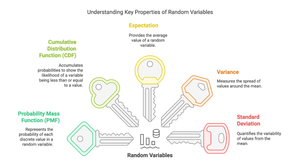
• Probability Distributions: Describe the likelihood of each possible value for a random variable using Probability Mass Functions (PMF) or Cumulative Distribution Functions (CDF).
• Key Characteristics: Expectation (mean) and Variance (spread) summarize the central tendency and variability of a random variable.
• Discrete Distributions: Specific models like Bernoulli, Binomial, and Poisson describe common discrete random processes (single trials, multiple trials, rare events).
• Independence & Combinations: Properties of sums or linear combinations of independent random variables can be derived from individual variable properties.

Definitions

• Random Variable (RV): A variable whose value is a numerical outcome of a random phenomenon. Typically denoted by an uppercase letter (e.g., X).
• Probability Mass Function (PMF): For a discrete RV, a function f(x) = P(X=x) that gives the probability that the RV X takes on a specific value x.
• Cumulative Distribution Function (CDF): A function F(x) = P(X ≤ x) that gives the probability that the RV X takes on a value less than or equal to x.
• Tail Probability: The probability that an RV X takes on a value greater than x, calculated as P(X > x) = 1 - F(x).
• Expectation (Mean, E[X] or μ): The weighted average of the possible values of an RV, where weights are the probabilities. Represents the long-run average value.
• Variance (Var(X) or σ²): The expectation of the squared deviation of an RV from its mean, E[(X - μ)²]. Measures the spread or dispersion of the distribution.
• Standard Deviation (SD or σ): The square root of the variance, providing a measure of spread in the original units of the RV.

Random Variables (General Properties)

Definition

A function that assigns a numerical value to each outcome in the sample space of a random experiment.

Key Insights

• The PMF, f(x), specifies the probability P(X=x) for each possible discrete value x. The sum of all PMF values must equal 1.
• The CDF, F(x), accumulates probabilities, representing P(X ≤ x). It is non-decreasing, starting at 0 and ending at 1.
• Expectation provides the central point or average value of the distribution.
• Variance quantifies the average squared distance of values from the mean, indicating variability. Standard deviation is the square root of variance.

Formula

• Expectation (Discrete RV): E[X] = Σ [x * P(X=x)] = Σ [x * f(x)]
• Variance (Discrete RV): Var(X) = E[(X - E[X])²] = Σ [(x - E[X])² * f(x)] Alternatively: Var(X) = E[X²] - (E[X])²
• Standard Deviation: SD(X) = √Var(X)
• Linear Combinations: If X₁, ..., Xₙ are independent RVs with E[Xᵢ] = μ and Var(Xᵢ) = σ², and S = ΣXᵢ:
  • E[S] = Σ E[Xᵢ] = nμ
  • Var(S) = Σ Var(Xᵢ) = nσ² (due to independence)

Bernoulli Distribution

Bernoulli Distribution - Definition

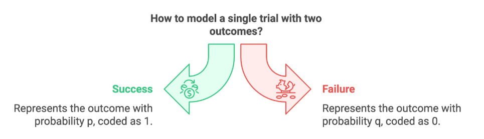
Models a single trial with exactly two possible outcomes, conventionally labeled "success" (usually coded as 1) and "failure" (usually coded as 0).

Bernoulli Distribution - Key Insights

• Characterized by a single parameter, p, the probability of success.
• The probability of failure is q = 1 - p.
• It is the fundamental building block for the Binomial distribution.

Bernoulli Distribution - Examples

• A single coin toss (Heads/Tails).
• The outcome of a single customer call (Purchase/No Purchase).
• Testing a single item (Defective/Not Defective).

Bernoulli Distribution - Formula

• PMF: f(y; p) = pʸ * (1-p)¹⁻ʸ, for y ∈ {0, 1} Alternatively: P(Y=1) = p, P(Y=0) = 1-p = q
• Expectation: E[Y] = p
• Variance: Var(Y) = p(1-p) = pq

Binomial Distribution

Binomial Distribution - Definition

Models the number of successes (y) in a fixed number (n) of independent and identical Bernoulli trials, where the probability of success (p) is constant for each trial.

Binomial Distribution - Key Insights

• Requires parameters n (number of trials) and p (probability of success per trial).
• Assumes trials are independent and have the same success probability.
• Represents the sum of n independent Bernoulli(p) random variables.
• Tools like MS Excel (BINOM.DIST function) can compute PMF (P(Y=y)) and CDF (P(Y≤y)) values.

Binomial Distribution - Examples

• Number of heads in 10 coin tosses (n=10, p=0.5).
• Number of successful insurance sales in 50 calls (n=50, p=estimated success rate).
• Number of defective pumps found in a daily sample of 20 (n=20, p=defect rate, "success" defined as finding a defect).

Binomial Distribution - Comparisons

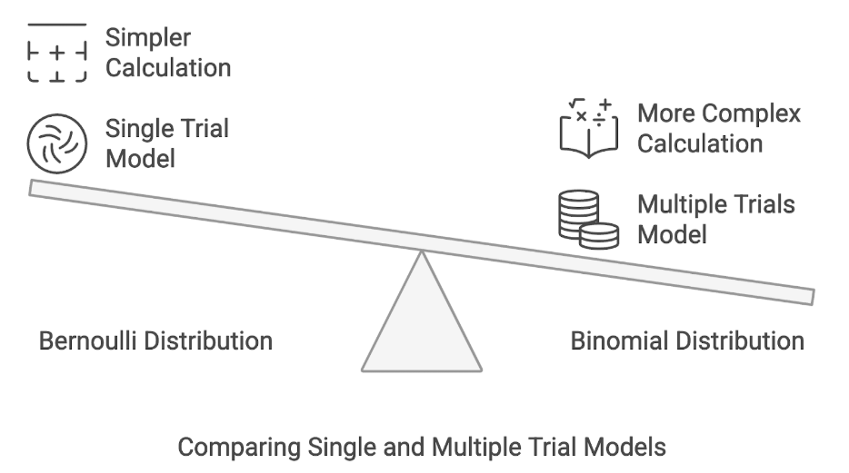
• Bernoulli vs. Binomial: Bernoulli models a single trial (n=1), while Binomial models multiple trials (n > 1).

Binomial Distribution - Formula

• PMF: f(y; n, p) = P(Y=y) = C(n, y) * pʸ * (1-p)ⁿ⁻ʸ where C(n, y) = n! / (y!(n-y)!) is the binomial coefficient ("n choose y"), for y = 0, 1, ..., n.
• Expectation: E[Y] = np
• Variance: Var(Y) = np(1-p) = npq
• Standard Deviation: SD(Y) = √[np(1-p)] = √[npq]

Poisson Distribution

Poisson Distribution - Definition

Models the probability of a given number of events (y) occurring within a fixed interval of time, space, or other continuous measure, when these events occur independently at a constant average rate. Often used for rare events.

Poisson Distribution - Key Insights

• Characterized by a single parameter, λ (lambda), representing the average number of events in the specified interval (the rate).
• The random variable Y can take non-negative integer values (0, 1, 2, ...).
• A key property is that the mean and variance are both equal to λ.
• Related to the Poisson process, where inter-arrival times between events follow an Exponential distribution. The count of events up to time t, N(t), in such a process follows a Poisson distribution with parameter λt (if λ is the rate per unit time).

Poisson Distribution - Examples

• Number of emails received per hour.
• Number of defects per square meter of fabric.
• Number of customer arrivals at a service counter per 10 minutes.
• Number of likes on a social media post per day.

Poisson Distribution - Comparisons

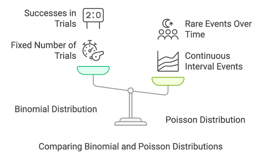
• Binomial vs. Poisson: Binomial counts successes in a fixed number of trials (n). Poisson counts events over a continuous interval (no fixed n), often applicable when n is very large and p is very small such that np ≈ λ.

Poisson Distribution - Formula

• PMF: f(y; λ) = P(Y=y) = (e⁻ˡ * λʸ) / y! where e is the base of the natural logarithm (≈ 2.71828), for y = 0, 1, 2, ...
• Expectation: E[Y] = λ
• Variance: Var(Y) = λ
• Standard Deviation: SD(Y) = √λ

Conclusion

This module introduces the foundational concept of random variables for quantifying uncertainty, characterized by their probability distributions (PMF/CDF), expectation, and variance. Building on this, three key discrete distributions are detailed: the Bernoulli for single two-outcome trials, the Binomial for counting successes across multiple independent Bernoulli trials, and the Poisson for modeling the occurrence of rare events over continuous intervals. Understanding these distributions and their properties (like the relationship between Binomial and Bernoulli, or the mean-variance equality in Poisson) is essential for analyzing probabilistic scenarios in various fields.