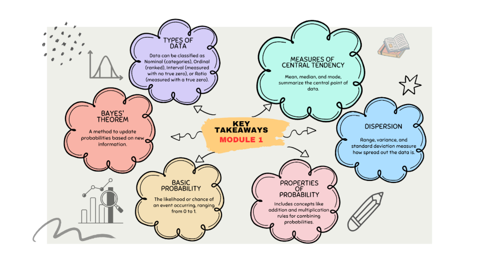
Core Concepts

• Descriptive statistics provides tools to summarize and describe data using numerical measures and visualizations, aiding decision-making.
• The type of data (qualitative vs. quantitative; nominal, ordinal, interval, ratio) dictates the appropriate statistical methods and visualization techniques.
• Data visualization techniques like frequency distributions, bar charts, histograms, and scatter plots help reveal patterns and relationships within data.
• Numerical summaries include measures of central tendency (mean, median, mode) to locate the center of the data and measures of dispersion (range, variance, standard deviation) to quantify its spread.
• Basic probability concepts provide a framework for understanding and quantifying uncertainty, which is essential for business forecasting and decision-making.

Definitions of Key Terms

• Statistics: Can refer to numerical facts (e.g., average, percentage) computed from data or the science/art of collecting, analyzing, presenting, and interpreting data.
• Descriptive Statistics: Methods involving organizing, summarizing, and presenting data in an informative way, using numerical measures and graphical tools.
• Elements: The entities on which data are collected (e.g., customers, companies, households).
• Variable: A characteristic of interest for the elements (e.g., age, income, satisfaction level).
• Observation: The set of measurements obtained for a particular element across all variables.
• Qualitative Data: Data represented by labels or names, identifying categories (numeric or non-numeric).
• Quantitative Data: Data represented by numerical values indicating "how much" or "how many".
• Cross-Sectional Data: Data collected at approximately the same point in time.
• Time Series Data: Data collected over several time periods.
• Random Experiment: A process that generates well-defined outcomes (e.g., rolling a die).
• Sample Space: The set of all possible outcomes of a random experiment.
• Event: A collection (subset) of outcomes from the sample space.
• Probability: A numerical measure of the likelihood that an event will occur, ranging from 0 to 1.

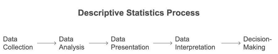
Introduction to Descriptive Statistics

Introduction - Definition

The practice of using numerical and graphical methods to describe, summarize, and present collected data effectively for interpretation and decision-making.

Introduction - Key Insights

• Statistics serves dual roles: as computed numerical facts and as a systematic process.
• This process involves collecting, analyzing, presenting, and interpreting data – considered both a science and an art.
• This module lays the groundwork for subsequent modules by covering fundamental data types, visualization, numerical summaries, and probability.

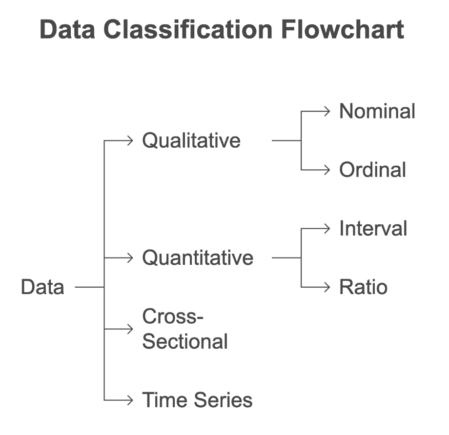
Types of Data

Types of Data - Definition

The classification of data based on its nature and measurement properties, which influences the choice of statistical analysis and visualization methods.

Types of Data - Key Insights

• Data can be broadly categorized as Qualitative or Quantitative.
• Data can also be classified based on the time dimension: Cross-Sectional or Time Series.
• The method of data collection (Observational vs. Experimental study) is another important consideration, with experimental studies often involving controlled conditions.

Types of Data - Examples

• Qualitative:
  • Nominal: Gender (Male/Female), Brand (Apple/Samsung), Operating System (Windows/MacOS/Linux). Categories have no inherent order.
  • Ordinal: Satisfaction Rating (Low/Medium/High), RAM Size (16GB/32GB/64GB). Categories have a meaningful order, but intervals between them may not be equal.
• Quantitative:
  • Interval: Test Scores (e.g., SAT scores), Temperature in Celsius/Fahrenheit, GPA (e.g., on a 2-10 scale). Ordered values with meaningful intervals, but no true zero point (0 does not mean absence). Ratios are not meaningful (e.g., 80F is not twice as hot as 40F).
  • Ratio: Age, Salary, Price, Square Footage, Number of Bathrooms. Ordered values, meaningful intervals, and a true zero point (0 means absence of the quantity). Ratios are meaningful (e.g., $100K salary is twice$50K).
• Cross-Sectional: Survey results of customer satisfaction collected in December.
• Time Series: Monthly sales figures recorded over the past two years.

Types of Data - Comparisons

• Qualitative vs. Quantitative: Qualitative describes categories; Quantitative describes amounts or counts.
• Nominal vs. Ordinal: Both are categorical. Nominal has no order; Ordinal has a meaningful order.
• Interval vs. Ratio: Both are quantitative with meaningful intervals. Interval lacks a true zero; Ratio has a true zero, allowing for meaningful ratio comparisons.

Data Visualization

Data Visualization - Definition

The use of tabular summaries (like frequency distributions) and graphical representations (like charts and plots) to explore, understand, and communicate insights from data.

Data Visualization - Key Insights

• Frequency distributions tabulate how often values occur within defined categories or classes.
• Relative and percent frequencies provide proportional views of the distribution.
• Bar charts and pie charts are common for categorical data; bar charts are often preferred for easier comparison.
• Histograms (for quantitative data) require careful definition of class intervals (typically 5-10 equal-width classes). The shape of a histogram reveals the data's distribution.
• Scatter plots are used to visualize the relationship between two quantitative variables.
• Data dashboards consolidate multiple visualizations for monitoring performance and facilitating decisions.

Data Visualization - Examples

• Tabular: Frequency Distribution, Relative Frequency Distribution, Percent Frequency Distribution.
• Graphical (Categorical): Bar Chart, Pie Chart, Side-by-Side Bar Chart, Stacked Bar Chart.
• Graphical (Quantitative): Histogram, Scatter Plot.

Data Visualization - Formula

• Relative Frequency: Relative Frequency = Frequency of the Class / Total Number of Observations
• Percent Frequency: Percent Frequency = Relative Frequency * 100

Measures of Central Tendency

Measures of Central Tendency - Definition

Numerical values that describe the typical or central value around which data points tend to cluster.

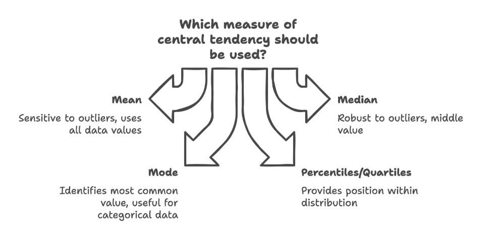
Measures of Central Tendency - Key Insights

• The mean is sensitive to extreme values (outliers), while the median is robust to them.
• The mode identifies the most common value(s) and can be used for categorical data.
• Percentiles and quartiles provide information about the position of values within the distribution. The median is the 50th percentile (Q2).

Measures of Central Tendency - Examples

• Mean: The arithmetic average.
• Median: The middle value in an ordered dataset.
• Mode: The most frequent value(s).
• Percentiles: The $p^{th}$ percentile is the value below which approximately $p$% of observations fall.
• Quartiles: Q1 (25th percentile), Q2 (50th percentile/Median), Q3 (75th percentile).

Measures of Central Tendency - Comparisons

• Mean vs. Median: The mean uses all data values and is affected by outliers. The median depends only on the middle value(s) and is less affected by outliers, making it preferable for skewed distributions.

Measures of Central Tendency - Formula

• Sample Mean ($\bar{x}$): $\bar{x} = \frac{\sum_{i=1}^{n} x_i}{n}$ (where $x_i$ are observations and $n$ is sample size)
• Population Mean ($\mu$): $\mu = \frac{\sum_{i=1}^{N} x_i}{N}$ (where $N$ is population size)

Measures of Dispersion

Measures of Dispersion - Definition

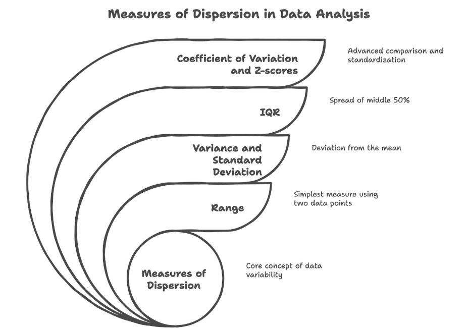
Numerical values that quantify the amount of variability, spread, or scatter within a dataset.

Measures of Dispersion - Key Insights

• Range is simple but only uses two data points.
• Variance and Standard Deviation measure the typical deviation from the mean. Standard Deviation is preferred as it's in the original data units.
• IQR measures the spread of the middle 50% of the data and is resistant to outliers.
• Coefficient of Variation allows comparison of variability between datasets with different means or units.
• Z-scores standardize data, indicating how many standard deviations an observation is from the mean, useful for comparing relative positions and identifying outliers.

Measures of Dispersion - Examples

• Range: Difference between maximum and minimum values.
• Variance: Average of squared deviations from the mean.
• Standard Deviation: Square root of variance.
• Interquartile Range (IQR): Q3 - Q1.
• Coefficient of Variation: Ratio of standard deviation to the mean (as a percentage).
• Z-score: Standardized value measuring distance from the mean in standard deviation units.

Measures of Dispersion - Formula

• Range: Range = Maximum Value - Minimum Value
• Sample Variance ($s^2$): $s^2 = \frac{\sum_{i=1}^{n} (x_i - \bar{x})^2}{n-1}$
• Sample Standard Deviation ($s$): $s = \sqrt{s^2}$
• Interquartile Range (IQR): IQR = Q3 - Q1
• Coefficient of Variation (CV): $CV = (s / \bar{x}) * 100\%$
• Z-score: $z = (x_i - \bar{x}) / s$ (for a sample observation $x_i$)

Five Number Summary and Box Plot

Five Number Summary and Box Plot - Definition

A method combining a concise numerical summary with a graphical representation to describe key features of a distribution.

Five Number Summary and Box Plot - Key Insights

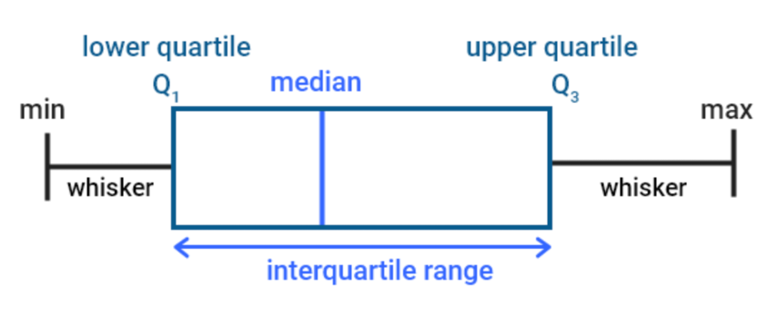
• The five number summary includes: Minimum, Q1, Median (Q2), Q3, Maximum.
• A Box Plot (or Box and Whisker Plot) visually displays the five number summary.
• The box represents the IQR (Q1 to Q3), the line inside the box is the median.
• Whiskers typically extend to the minimum/maximum values within a certain range (e.g., 1.5 * IQR) or to the actual min/max if no outliers are detected beyond that range.
• Box plots effectively show centrality (median), spread (IQR, range), skewness (median position within the box, whisker lengths), and potential outliers (points beyond the whiskers).

Five Number Summary and Box Plot - Examples

• Five Number Summary: {Min, Q1, Median, Q3, Max}
• Graphical: Box Plot

Descriptive Statistics Using Analysis ToolPak

Descriptive Statistics Using Analysis ToolPak - Definition

Leveraging the Data Analysis add-in in Microsoft Excel to efficiently compute a range of descriptive statistics for a dataset.

Descriptive Statistics Using Analysis ToolPak - Key Insights

• Provides a quick and automated way to obtain key summary statistics.
• Output includes measures like Mean, Median, Mode, Standard Deviation, Variance, Range, Min, Max, Sum, Count, etc.

Basic Probability

Basic Probability - Definition

The branch of mathematics concerned with analyzing random phenomena and quantifying the likelihood of events occurring.

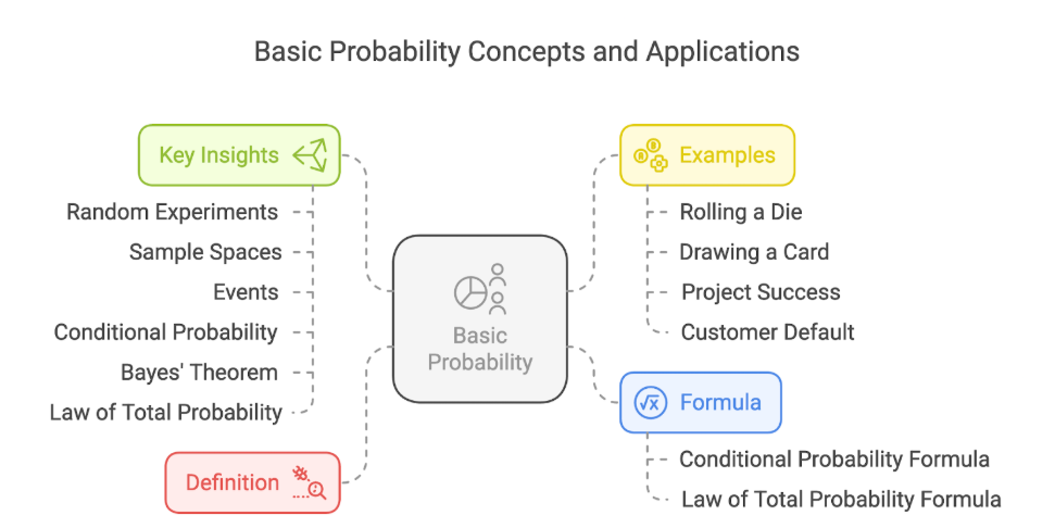
Basic Probability - Key Insights

• Foundation for statistical inference and decision-making under uncertainty.
• Involves understanding random experiments, sample spaces, and events.
• Basic probability rules: $0 \le P(E) \le 1$ for any event E; Sum of probabilities for all possible outcomes in the sample space equals 1.
• Concepts like union (A or B) and intersection (A and B) describe relationships between events.
• Conditional probability ($P(A|B)$) assesses the likelihood of event A given that event B has occurred.
• Bayes' Theorem provides a systematic way to update probabilities based on new evidence.
• The Law of Total Probability calculates the probability of an event by considering all mutually exclusive scenarios leading to it.

Basic Probability - Examples

• Determining the probability of getting a certain number when rolling a die (Random Experiment, Outcome, Sample Space).
• Calculating the probability of drawing a specific card from a deck (Event).
• Assessing the probability of a project succeeding given favorable market research (Conditional Probability).
• Updating the likelihood of a customer defaulting based on their payment history (Bayes' Theorem application, e.g., spam filters).

Basic Probability - Formula

• Conditional Probability: $P(A|B) = \frac{P(A \cap B)}{P(B)}$ (assuming $P(B) > 0$)
• Law of Total Probability: $P(A) = \sum_{i} P(A|B_i)P(B_i)$ (where $B_i$ are mutually exclusive and collectively exhaustive events)

Conclusion

Module 1 establishes the crucial role of descriptive statistics in business. It introduces methods for organizing data (types of data), summarizing it visually (data visualization), and numerically describing its central tendency and dispersion. Understanding these descriptive techniques, along with the fundamental concepts of probability, provides entrepreneurs with the essential tools to interpret data effectively and make more informed decisions in the face of uncertainty, setting the stage for more advanced statistical analysis in subsequent modules.